Most graph clustering methods fail because they ignore the network's shape, focusing only on node data. DGCSD solves this by using structural "seeds" to guide a Graph Neural Network, marking the first time seed detection and GNNs have been combined for clustering. By integrating both connection patterns and node features across its entire pipeline, the model creates sharper, more accurate groups. It is a competitive, open-source approach that proves understanding how nodes are connected is just as vital as knowing what they are.

Clustering Graphs with Seeds: Introducing DGCSD

(This is a summary of my published article at the Main Track of BRACIS 2025)

All the code from this project is available at GitHub

Graphs are everywhere, from social networks to the way traffic flows through a city. But making sense of this data is hard because we have to look at both the connections (topology) and the details of the nodes themselves (features).

While Graph Neural Networks (GNNs) are the go-to tool for this, most current clustering methods have a "disconnect" problem: they either learn the data and cluster it separately, or they ignore the graph's shape when trying to find group leaders.

The Problem: Missing the Big Picture

The Two-Step Gap: Many models learn node patterns first and cluster later (using K-Means). This means the model isn't actually "thinking" about clusters while it learns.
The Topology Blindspot: Some models pick "representative nodes" to guide clustering, but they often only look at node details, ignoring how those nodes are positioned in the network.

Our Solution: DGCSD

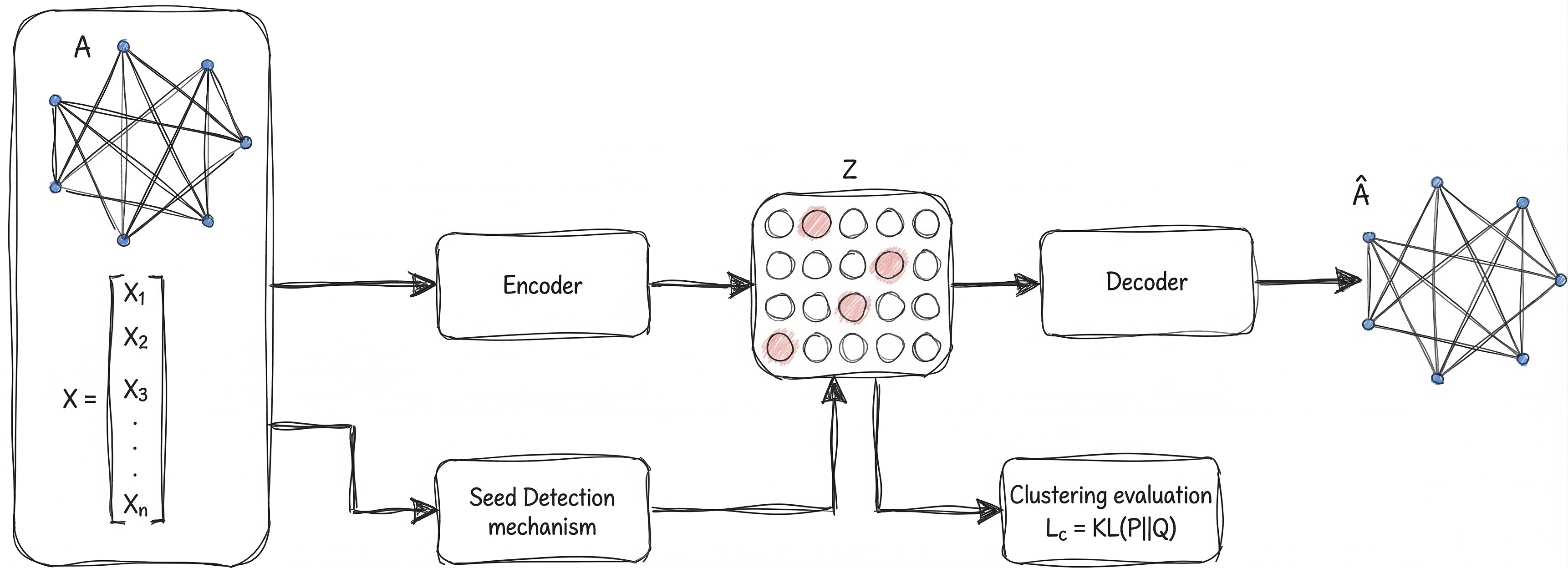
I developed DGCSD (Deep Graph Clustering with Seed Detection). It’s a framework designed to bridge these gaps using three specific modules:

Seed Detection: Instead of random guessing, we use "Centrality" (like how many paths pass through a node) to find the true structural leaders of a group.
The Embedding Engine: We use a Graph Autoencoder with Attention. This helps the model focus on the most important relationships between these central nodes.
Smart Refinement: We use a mathematical "nudge" (KL Divergence) to ensure the model's predictions align with the actual clusters it's discovering in real-time.

Why it Matters

Best of Both Worlds: It combines the graph's shape with the node's data.
Discriminative Learning: The model produces much sharper "boundaries" between different groups.
Open Source: I’ve released the toolkit so others can experiment with seed-based clustering.

In our tests against state-of-the-art algorithms, DGCSD showed it could compete with—and often outperform—traditional methods by being smarter about how it "plants the seeds" for clusters.

The Landscape: How Others Do It

In the world of Graph Neural Networks (GNNs), there are two main ways to group data. Think of it as the difference between a two-step DIY project and an "all-in-one" automated system.

1. The "Map then Group" Strategy (Embedding Models)

Most researchers use a two-step process. First, they use a Graph Autoencoder to compress the complex network into a simpler "latent space", basically a digital map where similar nodes sit closer together. Once the map is ready, they use a standard tool like K-Means to draw circles around the groups.

The Problem: The AI builds the map without knowing where the clusters are supposed to be. It’s like packing a suitcase without knowing if you're going to the beach or the mountains, you might leave out the most important details.

2. The "All-in-One" Strategy (Deep Models)

These models are more ambitious; they try to learn the map and the clusters at the same time. There are two ways to guide them:

The Math Route: Using a specific formula (like "Modularity") to score how well the groups are forming. It sounds great, but finding a formula that works for every type of graph is notoriously difficult.
The "Follow the Leader" Route: This is where the model picks a few "representative nodes" (seeds) to act as the center of each group. These seeds guide the rest of the nodes into the right clusters.

Where DGCSD Fits In

Existing "Follow the Leader" models (like DNENC) usually pick their seeds based only on node data, like grouping people in a social network solely by their age.

DGCSD changes the game by looking at the social ladder (the graph structure) too. We find the most "central" nodes to act as seeds, ensuring the model understands both who the nodes are and how they are connected.

Inside the Engine: How DGCSD Works

DGCSD isn't just another clustering algorithm; it’s a three-act play. Instead of guessing where groups start, we find the "influencers" of the graph first and let them lead the way.

Module 1: The Seed Detectors (The Anchors)

Most models use K-Means to find centers, but K-Means is "graph-blind." We replaced it with Seed Detection. We identify the most important nodes using network math:

Betweenness Centrality: Finding the "bridges" that connect different parts of the graph.
Closeness Centrality: Finding the nodes that are "hops" away from everyone else.
Random Seeds: A baseline to see if the structure actually beats luck (spoiler: it does).

These seeds act as fixed anchors, giving the GNN a massive head start in understanding the graph’s layout.

Module 2: The Embedding GAE (The Map Maker)

Once we have our anchors, we use a Graph Autoencoder (GAE). Its job is to take high-dimensional data and squash it into a low-dimensional "latent space."

The Encoder: Looks at node features and who is talking to whom.
The Decoder: Tries to "reconstruct" the original graph from the squashed version.

If the decoder can rebuild the graph, it proves the encoder successfully captured the most important patterns.

Module 3: Self-Supervised Refinement (The Polisher)

This is where the magic happens. We don't just stop at a pretty map; we run a joint optimization. The model tries to do two things at once: 1. Keep the graph structure accurate (Reconstruction Loss). 2. Pull nodes closer to their assigned seeds (Clustering Loss).

By balancing these two goals, the clusters become tighter and the boundaries between groups become much sharper.

DGCSD - How it works.

The Seed Detection Module: Finding the "Founding Members"

In graph clustering, you need a starting point. Most algorithms pick these starting points (centroids) randomly or based only on node data. DGCSD does something different: it uses Seed Detection to find the most structurally influential nodes to lead each cluster.

Think of these "seeds" as the founding members of a community. If we pick the right leaders, the rest of the group organizes itself much more naturally.

The Math of Influence

We represent our network as $G = (V, E)$, where $V$ are the nodes and $E$ are the connections. Every node also has a feature vector $\mathbf{x}_i$ (the data it carries).

Our goal is to find a set of $k$ seeds ($U^*$) that maximizes a specific "influence score" $c(v)$:

$$U^* = \arg\max_{U \subseteq V,\, |U|=k} \sum_{v \in U} c(v)$$

Three Ways to Pick a Leader

We tested three different strategies to see which structural metric guides the GNN best:

1. Betweenness Centrality (The "Bridges")

This measures how often a node acts as a bridge along the shortest path between other nodes.

The Logic: If a node sits on many "shortcuts," it likely connects different regions of a cluster.
The Formula: $BC(v) = \sum_{s \neq v \neq t} \frac{\sigma_{st}(v)}{\sigma_{st}}$ (where $\sigma$ is the number of shortest paths).

2. Closeness Centrality (The "Hubs")

This measures how "close" a node is to everyone else in the network.

The Logic: A node with high closeness can reach the entire cluster quickly. These are the centers of gravity for a group.
The Formula: $CC(v) = \frac{|V|-1}{\sum d(v,u)}$ (where $d$ is the distance between nodes).

3. Random Seeds (The Baseline)

We pick nodes at random to act as seeds. This helps us prove that using the graph's math (like BC or CC) actually provides a better "map" than just luck.

Why this matters for the GNN

By identifying these seeds first, we give the GNN a "ground truth" to aim for. Instead of wandering aimlessly through the data, the model's loss function calculates the distance between every node and these high-influence seeds, forcing the network to learn a much more organized structure from the very first epoch.

The Tech Stack: Creating Better Embeddings

To group nodes effectively, we need to turn a complex web of connections into simple coordinates. We do this in two stages: Encoding and Refining.

1. The Embedding Module (The Map Maker)

We use a Graph Autoencoder (GAE) to compress the graph. Think of this as taking a giant, messy 3D sculpture and finding the perfect 2D shadow that still shows all the important details.

The formula for this "compression" (the Encoder) is: $$Z = \sigma(\tilde{A}XW)$$

$\tilde{A}$ (The Connections): Who is connected to whom.
$X$ (The Data): What each node actually contains.
$W$ (The Brain): The weights the model learns during training.
$Z$ (The Result): A clean, low-dimensional "latent space" where the clustering happens.

2. The Secret Sauce: Multi-Hop Neighborhoods

Standard models only look at a node’s immediate neighbors. In DGCSD, we look further. We use a transition matrix $B$ (which calculates the probability of a "random walk" from one node to another) to build a Multi-hop Matrix ($M$):

$$M = (B + B^2 + \dots + B^t) \cdot t$$

By looking at $t$-hop neighbors, the model understands the broader "neighborhood" context, not just the guy next door. This makes the clusters much more accurate.

3. Self-Supervision: The Feedback Loop

To make sure our clusters are tight and distinct, we use a dual-loss function: $$L = L_r + \gamma \cdot L_c$$

Reconstruction Loss ($L_r$): Ensures the model doesn't "forget" the original graph structure.
Clustering Loss ($L_c$): Uses KL Divergence to nudge nodes toward their cluster centers.

How the "Nudge" Works

We calculate two distributions:

$Q$: How close a node actually is to a cluster center (using a t-Student distribution).
$P$: The "ideal" target distribution where nodes are perfectly grouped.

By minimizing the difference between $Q$ and $P$ ($KL(P \parallel Q)$), the model essentially "self-corrects" until the clusters are as sharp and cohesive as possible.

Wrapping Up: The Future of Graph Clustering

With DGCSD, we’ve bridged the gap between "old-school" graph theory and cutting-edge Deep Learning. By treating structural seeds as a compass, we’ve turned a blind, unsupervised clustering problem into a guided, self-supervised success story. You can see some of the results in the image bellow:

DGCSD - Some results.

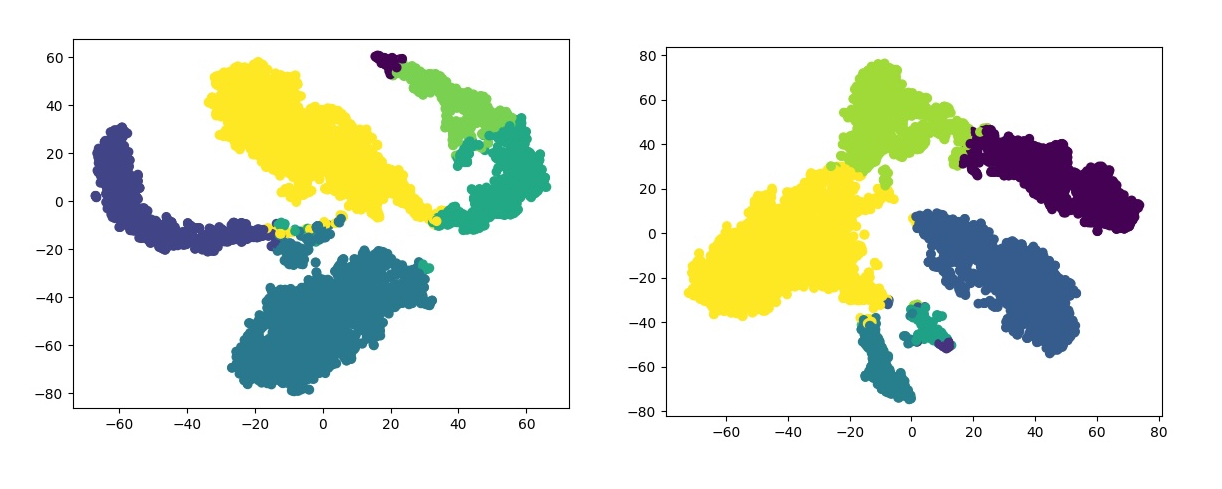
The Bottom Line

Instead of letting a Graph Neural Network wander aimlessly through data, we anchored it with structural "leaders" (seeds). This joint approach, balancing graph reconstruction with cluster cohesion, doesn't just produce cleaner data; it produces groups that actually make sense in the real world.

Our experiments prove that this isn't just a theory. DGCSD holds its own against state-of-the-art algorithms, showing that the shape of the graph is just as important as the data within it. All the detailed comparisons with other popular algorithns can be found in the original published article.

What’s Next?

This is just the beginning. The next steps for this project include:

Scaling Up: Testing the framework on massive, real-world datasets with millions of nodes.
Adaptive Seeds: Moving from fixed seed selection to "smart" seeds that adapt as the model learns.
New Architectures: Experimenting with different GNN layers to see how far we can push the accuracy boundaries.

Deep graph clustering using Graph Neural Networks and Seed Detection